

Trespasser - C++ archeology and oxidization - Part 1 Loading Scene Data
This series will be about the video game Jurassic Park Trespasser. My goal is to be able to play the game by rewriting its source code in Rust based on the original C++ code base. Hopefully discovering interesting things along the way.
Why this project?
Not sure why I like this game, I only played it properly once, never finished it but I was amazed by the technical aspects of it. Even with all the technical issues, I’m sure all the fans will agree that being chased by a clumsy raptor while trying to wrangle a rifle with one hand is an experience that only this game can give.
For this project, I decided to go back to Rust after trying it for Advent of Code a few years ago and failing to grasp its concepts in the short allocated time for the puzzles. This time around, I have time to read the documentation and understand what I’m doing wrong. It also helps that the tools have immensily improved like the LSP server for VS Code which is great for writing in a language you don’t know well enough yet. The game was developed with compilers that didn’t understand the standard very well yet and lots of workarounds had to be added.
For more background on the game, I would recommend these links:
- Fabien Sanglard’s Source Code Review: https://fabiensanglard.net/trespasser/
- Joueur du Grenier: https://www.youtube.com/watch?v=WVE_yU38YVI
- Angry Video Game Nerd: https://www.youtube.com/watch?v=15pi8vrUx9c
In this part, we’re going to explore some file formats with the goal of trying to display some of the geometry data from the game.

Scenes
SCN files
The BE.SCN file is the one we’re going to start with. It’s a natural start as it’s the one referenced from the “New Game” menu in the game:
|
|
Following the LoadLevel call, we can find an interesting piece of code:
|
|
A CSaveFile instance reads the header of a .SCN file and extracts the header which contains the list of .GRF files to load.
|
|
Note that we’ve actually been dealing with what’s called a GROFF file structure in .SCN files. A GROFF structure is organized like this:
|
|
We can see from this that we have a magic number (always 0x0ACEBABE), a list of sections and a list of symbols. Each section has a symbol handle and data. To read the header SSaveHeader above, we need to read the .SCN file with the GROFF parser and then read the section named Header which contains the byte stream we’re interested in. Replicating this in Rust gives us this output:
|
|
The number of GROFF files and the length of their names is hardcoded, in this case we’ll just need to load BE.GRF. It is stored as a full path here, but the code looks for the base name in a few folders so it just works.
GRF files
As expected BE.GRF is a GROFF file. However, when opening it in a hex editor, it doesn’t start with BE BA CE 0A, but it starts with SZDD in ASCII. A quick search shows that it’s the compression format used by the DOS utility named COMPRESS.EXE as well as the LZOpen/LZRead Windows APIs which is what the game used at runtime.
I used this page as a reference to implement my own decompressor which implements the Rust Read trait and can be chained with the other parsers if needed. Here is the decompressor pseudo-code from the page:
|
|
The Rust code I’ve written follows the pseudo-code from the link above very closely and works perfectly to be able to decompress .GRF files:
|
|
Because we already had GROFF parsing done for the .SCN files, we can now load compressed .GRF files using the same code because we implemented the Read trait.
.GRF files follow the GROFF structure but also contain additional info that points us to the right sections to read for example. We have a list of CGroffObjectConfig for example:
|
|
We can then look up an object by its name, load the data from its section and look up attributes in the value table. At this point, I had enough to be able to write this in Rust:
|
|
Which outputs this:
|
|
I thought that each CTerrainObj would contain a mesh for each part of the terrain. However, that was before I remembered the part of Fabien Sanglard’s article where he describes the terrain as using a wavelet transform to store heightfield data. I still wrote the code to load meshes so here is an example of a mesh:

I found while parsing meshes that they are polygonal meshes, some of them mostly composed of polygons instead of triangles. For example, this truck:
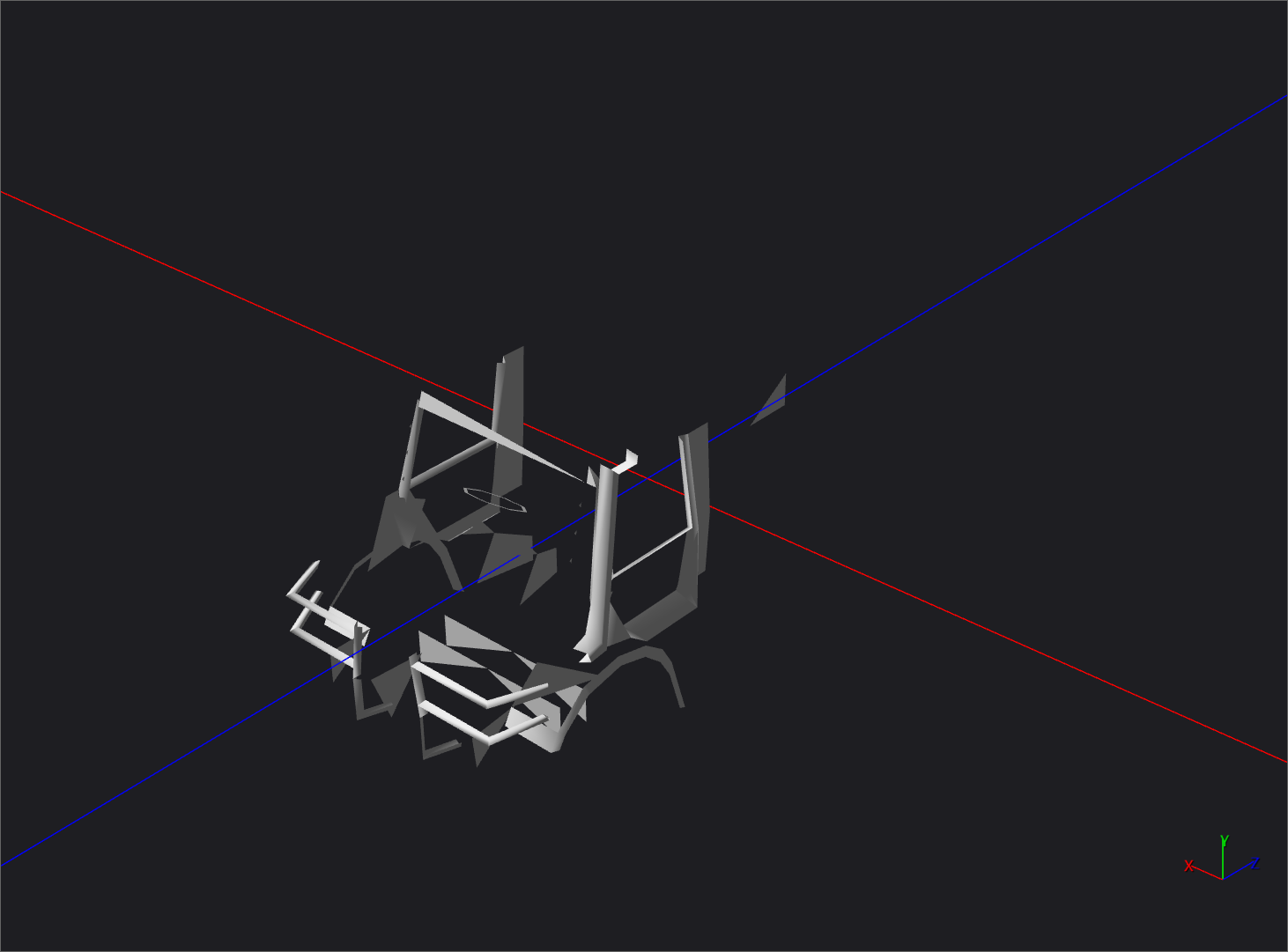
Triangles only
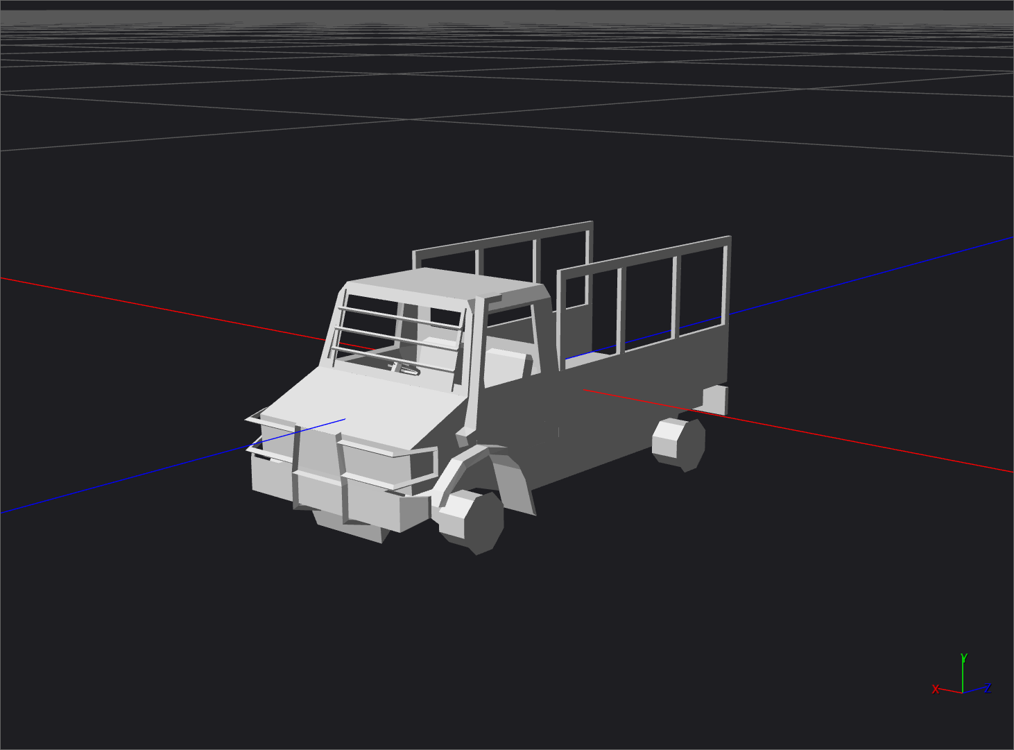
All polygons
Textures
PID files
These files are an “image directory”. It contains just a list of descriptors for each of the textures used in a level. It looks like this from C++:
|
|
Some members point to offsets into the next file format we’ll investigate. You’ll also notice that textures can be paletted which is quite common for space saving in games back then.
SPZ files
These files contain the actual data for the textures. They’re the biggest files in a level as you can see here:

And that’s also a compressed format! The uncompressed size is about 54.5MB. However, the format is slightly different than the SZDD one used for .GRF files. First, the header is custom and only consists of the uncompressed size as a u32. Second, the algorithm is the same with just a few setup parameters that are different:
- The start position inside the decompression window is different
- The window buffer is initialized to 0 instead of space characters
Looking at the SDirectoryFileChunk structure above, the value in u4VMOffset is actually an offset from the beginning of the uncompressed data from the .SPZ files. Because compressed data can’t be addressed this way, the original game would decompress the .SPZ files on demand and write out a .SWP file with the uncompressed data to the hard disk, and it’s that one that would be read for each texture.
However, for us, it’s now just easier to load and decompress the whole file in memory. We can then fetch the data using the u4VMOffset value into a [u8] in Rust.
The game supports mipmaps for textures. Each mipmap is hashed into a u64 value and the bottom 32 bits are shared between all the mips.

Example of a mipmap chain extracted from the game (256x256 to 8x8, zoomed 4x)
Terrain
The terrain data is constructed from a point cloud to start with, during authoring time exported to a .TRR file from 3DSMax. This is then compressed into a quad-tree with wavelet transform coefficients at each vertex. Vertices are shared between the quad tree nodes. For runtime, this data is saved into a .WTD file which has a small header and a list of every node, for each descendant node (a node is always subdivided into 4 at a time when required) a bit is stored to know if it has data and children to read.
The way this file is read is slightly different than other ones in that it loads the file data as an array of u32. Reads are done by specifying how many bits are needed, the twist is that these bits are read higher to lower from each u32. So, when looking at the file in a hex editor it doesn’t make much sense as you are mixing little-endian u32 values but their bytes are reversed. For example, writing 8 bytes from 0 to 7 gives 03 02 01 00 07 06 05 04 instead of the usual 00 01 02 03 04 05 06 07. With more complicated data, it was confusing at first.
From the C++ code, here are some interesting bits regarding the quad-tree code:
|
|
Here is a description of the wavelet coefficients:
|
|
To understand what this means, a look at Wikipedia gives us some clues:
From https://en.wikipedia.org/wiki/Cohen-Daubechies-Feauveau_wavelet#Numbering
The same wavelet may therefore be referred to as “CDF 9/7” (based on the filter sizes) or “biorthogonal 4, 4” (based on the vanishing moments). Similarly, the same wavelet may therefore be referred to as “CDF 5/3” (based on the filter sizes) or “biorthogonal 2, 2” (based on the vanishing moments).
In our case, the transform is also called “CDF 5/3”, and from the same Wikipedia page, we can confirm that it’s a lossless transform:
The JPEG 2000 compression standard uses the biorthogonal LeGall-Tabatabai (LGT) 5/3 wavelet (developed by D. Le Gall and Ali J. Tabatabai) for lossless compression and a CDF 9/7 wavelet for lossy compression.
I found a very interesting article and it helped me a lot to understand the basic theory. From https://georgemdallas.wordpress.com/2014/05/14/wavelets-4-dummies-signal-processing-fourier-transforms-and-heisenberg/
These waves are limited in time, whereas sin() and cos() are not because they continue forever. When a signal is deconstructed into wavelets rather than sin() and cos() it is called a Wavelet Transform. The graph that can be analysed after the transform is in the wavelet domain, rather than the frequency domain.
So when you use a Wavelet Transform the signal is deconstructed using the same wavelet at different scales, rather than the same sin() wave at different frequencies. As there are hundreds of different wavelets, there are hundreds of different transforms that are possible and therefore hundreds of different domains. However each domain has ‘scale’ on the x-axis rather than ‘frequency’, and provides better resolution in the time domain by being limited.
When searching for examples of a Discrete Wavelet Transform online, one of the reference materials often found is the dwt53.c example from Grégoire Pau. I ported it to JavaScript to make this visualization below.
The main take away I got from this is that with each transform, the original signal gets compressed into approximation coefficients and detail coefficients. The approximation coefficients once the transform is applied enough times, will have only one value left. The detail coefficients end up with values that make them more compressible and you’re able to compress the data more efficiently. For the terrain quad-tree nodes, that property is used to use less and less bits to store the wavelet coefficients depending on the subdivision level.
The Wikipedia example with an image shows that quite clearly:
![]()
After this interlude on wavelets, we can dig into parsing the BE.WTD file. Here is its header after parsing the file in Rust:
|
|
As you can see in the highlighted lines above, it contains the root coefficient, which is the one wavelet coefficient I was talking about. It also contains scales to transform to/from quad-tree coordinates and also to/from wavelet coefficients and world coordinates. That’s how the world Z value of each terrain vertex is obtained mesh from the integer wavelet coefficients.
For ease of porting for now, I decided to subdivide the quad-tree to the maximum possible to get the full resolution of the tree. In the original code, it would compute the best subdivision factor for each quad depending on the desired pixel density. Once I get to porting gameplay features, I’ll be able to reproduce that behaviour and query the player position, camera position, etc. to compute the original parameters to subdivide.
Finally, we can obtain a mesh of the fully subdivided terrain from the Rust code.


Conclusion
We have been able to read all the scene files that were available to us:
BE.SCN: references the.GRFfiles and contains some other basic scene informationBE.GRF: contains most of the scene data like entities, meshes, animations, triggers, etc.BE.PID+BE.SPZ: contains all the texture data, used as streaming format that would be temporarily expanded on the hard diskBE.WTD: wavelet compressed terrain data stored as quad-tree
Just from these files, we are able to reproduce a lot of the scene data. Glueing this data together to produce textured meshes placed on the terrain will be the next step in this series. See you soon!